Overview
This project is a full workflow exercise: take an imperfect public dataset and make it usable for regression modeling. The goal wasn’t “perfect accuracy” — it was to practice the real steps that decide whether ML is meaningful: consistent features, honest handling of anomalies, and clear evaluation.
What I built
A MATLAB pipeline for preprocessing + visualization + supervised regression, then benchmarking multiple learners (tree-based, linear, and kernel methods).
What it demonstrates
Data hygiene, feature design, and model comparison.
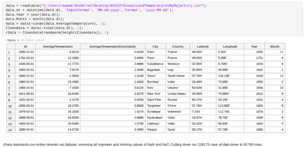
Data Prep
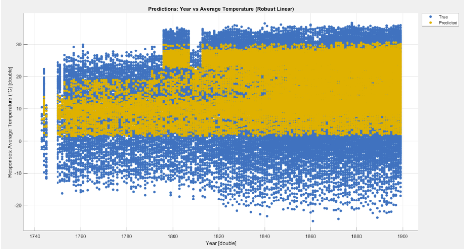
The dataset contained inconsistent timestamps (multiple date formats + missing entries), which forced the pipeline to explicitly decide: normalize dates into a consistent representation or engineer a simpler derived feature (e.g., Year) to keep the model stable.
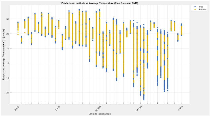
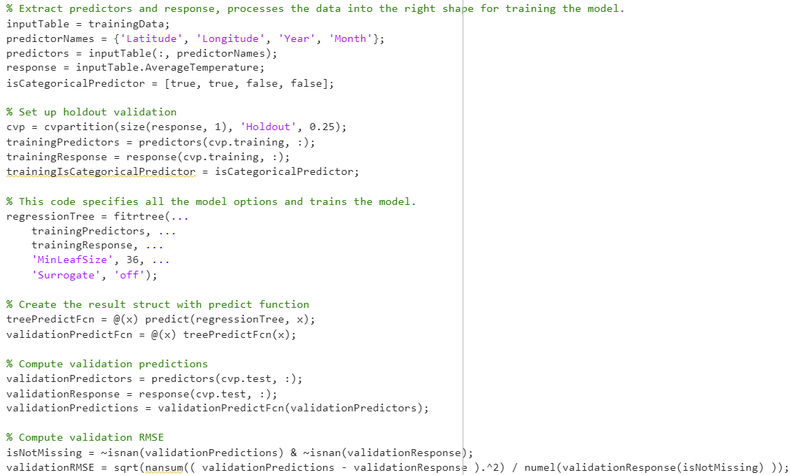
Key features used
Date/Year (temporal trend), AverageTemperature (target/response), and Latitude (geographic signal). This kept the model interpretable while still predictive.
Outliers: kept on purpose
Instead of deleting extreme points automatically, I preserved them when plausible climate data can include true anomalies (events, measurement artifacts, regime shifts).
One-Hot Encoding
Categorical and mixed-format fields needed to be converted into numeric features for regression. One-hot encoding let the model represent discrete labels without imposing fake ordering.
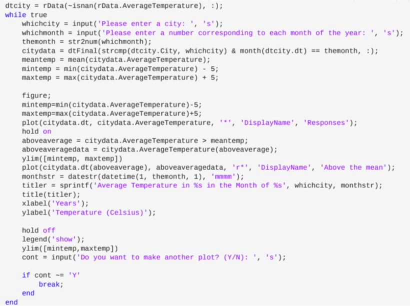
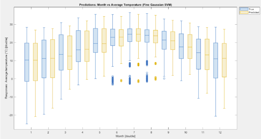
Interactive Plots
I wrote a MATLAB routine that repeatedly prompts for a city and month (1–12), then plots the selected temperature history. Points above the mean are highlighted to make “unusual” periods visually obvious. This created an easy way to compare cities across regions without manually slicing the dataset.
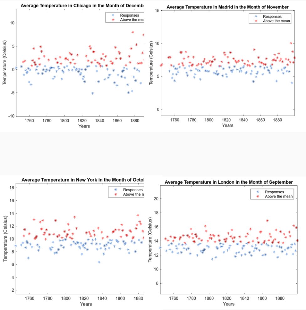
Why this mattered
Visualization caught issues early (bad slices, weird distributions, missing data), and made model results easier to sanity-check.
UI goal
Minimal friction: type a city + month → immediately see the story in the data.
Model Training
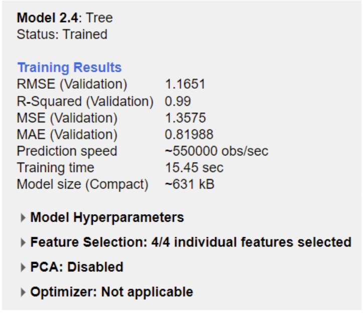
I treated this as a regression problem (predicting a continuous temperature value). I compared multiple learners in MATLAB’s Regression Learner and prioritized models that performed well while still being explainable.
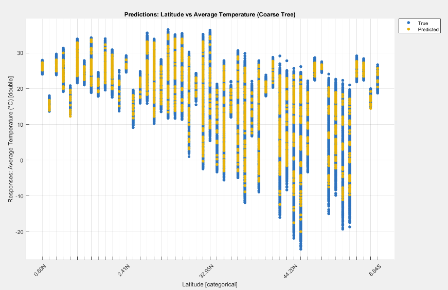
What worked best
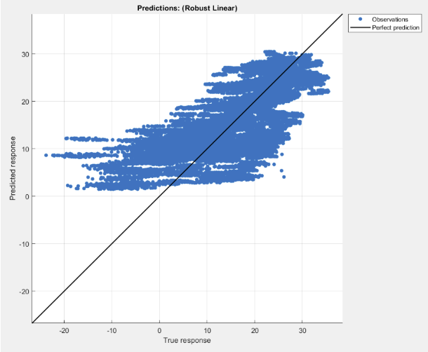
Tree-based models performed strongly, suggesting the relationship between features and temperature isn’t purely linear.
What I looked for
Error metrics, residual behavior, and consistency across slices — not just one “best score.”
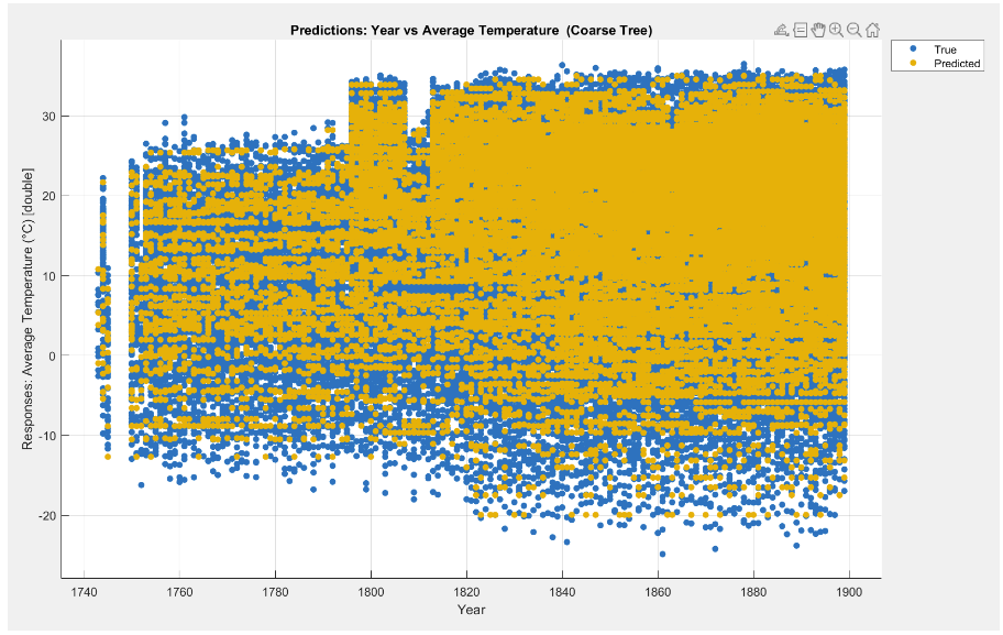
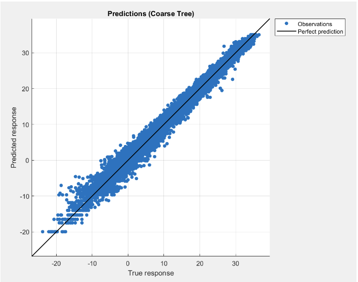
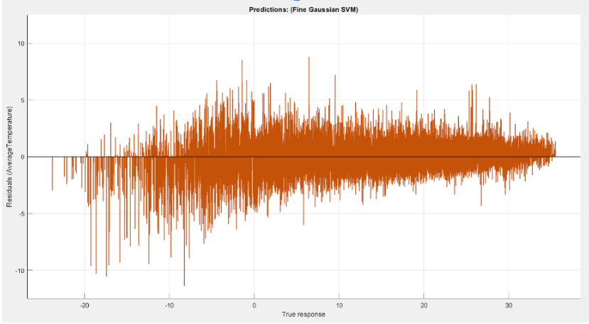
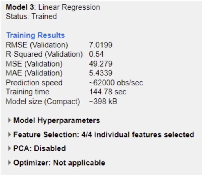
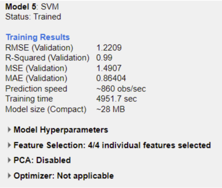
Results
The most consistent models captured nonlinear structure in the data and produced more stable residuals. Beyond the leaderboard, the bigger takeaway was how strongly performance depends on preprocessing quality and feature decisions.
Takeaway
Better features beat “more complex” models when the dataset is noisy or inconsistent.
Next improvement
Add richer geography features (region bins, hemisphere, elevation proxy) and validate using time-based splits (train on early years → test on later years).
Reflection
Challenges
• Long training times for heavier learners limited how many sweeps I could run.
• Feature formatting in MATLAB apps required careful conversions (categorical ↔ numeric ↔ cell).
• Dataset inconsistencies forced explicit tradeoffs instead of “auto-cleaning.”
What I learned
• How to structure a large preprocessing workflow that stays debuggable.
• How to compare regressors beyond one score (residuals, stability, sanity checks).
• Transferable habits for data work (feature design, slicing strategy, validation logic).
 by Justin Yu